Today I want to work through DQN, or Deep Q-Network, by reading Playing Atari with Deep Reinforcement Learning.
This is a landmark paper in reinforcement learning. It was also my first serious paper reading: at the time, I translated the entire paper myself. Before posting on Tistory, I prepared for a lab meeting in Notion and kept the feedback there. I have linked those rough original notes at the end.
For me, the most important questions in this paper are why combining deep learning with reinforcement learning was unstable, and which practical choices helped DQN make that combination work.
When I first read it, the equations were confusing. I even mixed up the exploration probability with the environment . The statement that “the target depends on the network” did not immediately make sense to me either. I will follow the paper's progression while spending extra time on the points that confused me and the ideas that eventually clicked.
So, what does DQN actually do? Let's get into it.
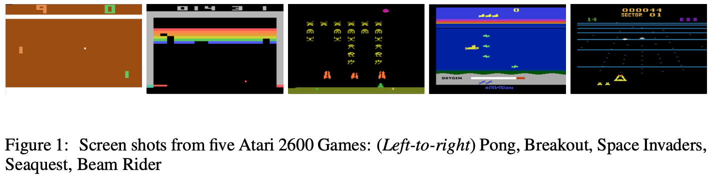
The reproduced Figure 1 and Algorithm 1 below come from Mnih et al. (2013), Playing Atari with Deep Reinforcement Learning. They are preserved as they appeared in my Korean article, without alteration. Copyright remains with the original rights holders; they are included here for discussion of the paper.
The problem DQN tried to solve
The paper begins with a question: can a reinforcement learning agent learn how to act directly from high-dimensional sensory input, such as images?
Earlier reinforcement learning systems often depended heavily on features designed by people. For a game, a person might process the screen into object positions, velocities, colors, or score information before giving it to the agent. Performance then depends strongly on the quality of those features.
Deep learning offered a different route. A CNN can learn useful visual representations from pixels: edges, shapes, and more complex patterns. Deep models had also shown that useful representations could be learned from speech signals.
Put simply, instead of manually extracting positions, velocities, and scores, we would give the model the game screen and let it learn useful representations itself. That leads to the natural question: could an RL agent learn both useful features and a good policy from raw pixels?
“Raw pixels” means the screen itself, rather than an externally prepared description of the game. DQN was an early, powerful answer to this question.
In the paper, the agent learns Atari 2600 games using screen images, reward signals, terminal signals, and the available actions. People do not design a separate visual feature set for each game. The significance is therefore more than a high score: the system learns action-values end to end from visual input.
Why is deep learning plus RL difficult?
The introduction explains why attaching a deep network to reinforcement learning is not straightforward. Understanding these difficulties is central to understanding the paper.
Supervised deep learning commonly starts with many labeled examples: an image, a correct label, and a learning objective that encourages the model to predict that label. Reinforcement learning has a different structure:
- Rewards can be sparse, noisy, and delayed.
- Successive observations can be strongly correlated.
- As the agent learns, its behavior changes the distribution of its own training data.
An action in an Atari game may not produce a useful reward immediately. Its consequences might become clear hundreds or thousands of steps later. Meanwhile, neighboring frames are almost identical: they form a sequence, rather than a collection of unrelated images.
The policy also determines which states the agent visits. When the policy changes, the observed data changes with it. The training distribution is therefore not fixed, a major difference from the usual supervised-learning setup.
At first, I also thought, “Can't we just put Q-learning on top of a CNN?” These difficulties explain why that is not the whole story.
Viewing Atari as a reinforcement learning problem
The paper treats the Atari emulator as the environment, written , and has the agent select an action at each time step.
A small notation warning, because I once confused these myself: is the environment; is the probability of choosing a random action. They play completely different roles. The first denotes the emulator; the second controls exploration in an -greedy policy.
The agent cannot inspect the emulator's internal state. It observes an image of the current screen, much as a human player does. This makes the task partially observed.
The paper calls attention to perceptual aliasing: different underlying situations can look the same in one image. For example, a single frame may show where a ball is without revealing whether it is moving left or right.
The paper first defines a state as the history of observations and actions. In the actual network, a preprocessing function turns that history into a fixed-size input using the most recent four frames. Stacking frames provides information about motion, although it does not guarantee access to the full hidden state.
Return and the Q-function
The agent wants to maximize the rewards it receives in the future. The paper defines the discounted return as
This adds rewards from the current time until the episode ends at , discounting rewards that arrive further in the future. The discount factor determines how much weight to give future rewards relative to immediate ones.
The optimal action-value function is
Starting in state , taking action , and then following the best possible policy, what is the largest expected return we can achieve?
In more everyday language: if I do this now, how good can things be from here onward?
DQN uses a neural network to approximate this .
What the Bellman equation says
The optimal Q-function satisfies the Bellman equation:
Taking action in state produces a reward and leads to the next state . From there, we choose the best available action.
The value of the current action is therefore the immediate reward plus the best discounted future value from the next state. That is the central idea behind Q-learning.
Written as value iteration, the update is
Under the usual assumptions for exact value iteration, repeatedly applying this update converges to . That theoretical result does not automatically carry over to a neural network trained on samples.
Atari has an enormous number of possible observation histories. Storing a separate Q-value for every state-action pair in a table is impractical. We need a function approximator, and DQN uses a neural network for that role.
The Q-network and the TD target
We write the network as
where denotes its weights. To train it, we need a target. The paper writes the loss as
with
The important quantity here is , the temporal-difference, or TD, target.
If this is your first paper, simply showing the equation is not much help. Reading the symbols was one of the hardest parts of my own first reading. I will unpack the loss in the next section; you can jump there and come back if that makes the flow easier.
At first, looks like a supervised-learning label. But supervised-learning labels are usually fixed before training begins. Here, the target includes a prediction made by the network at the next state. The target itself depends on network parameters.
This is one reason learning can become unstable. We use an estimate to construct another estimate, then update the network toward it. In my old Notion notes, this was the point where I wrote, “So this is the TD target.”
A detail matters when reading this particular paper: the loss derivation uses the preceding iteration's parameters and treats the target as fixed for that optimization. Algorithm 1 computes a sampled target with the current network weights before updating them. The 2013 algorithm does not maintain the separate, periodically copied target network associated with the later 2015 DQN. My Korean explanation used the later shorthand in one equation; here I keep the notation consistent with the paper being read.
So what exactly is that loss?
Let's look at the full expression again:
It says that we want the Q-network's prediction to approach a target value. We can read it one piece at a time.
1. The loss at iteration i
is the loss at learning iteration . It measures the prediction error when the network has parameters .
The loss is the quantity we want to reduce. A prediction close to its target gives a small loss; a prediction far from its target gives a larger one.
2. The network prediction
is the current Q-network's prediction for state and action : its estimate of the discounted reward available after taking that action.
The roles of and are different. The state and action identify the quantity being evaluated, while is the set of weights learned during training. The semicolon separates those roles.
The same value is sometimes written . The notation changes, but the meaning does not: it is the Q-value assigned by the network whose parameters are .
There is one more distinction that confused me: the difference between and .
In probability, normally means “given.” For example, means the probability of given . The semicolon in is a notational separator between the arguments being evaluated and the parameters that define the function. It is not itself a probabilistic conditioning operation.
One architectural detail will matter later: although we write the mathematical function as , DQN's network receives the state representation and outputs a Q-value for every available action. The action identifies which output we are referring to; it is not a second input fed into this particular architecture.
3. The target value
is the value we ask the current prediction to follow. For a sampled non-terminal transition, the 2013 algorithm uses
computed before the weight update and held fixed while taking that update. If the next state is terminal, the target is simply .
The non-terminal expression adds the reward just received to the largest predicted Q-value at the next state, discounted by .
It acts something like an answer to learn from, but it is not a perfect answer. We do not receive it entirely from outside the model. We build it using what the network currently believes about future rewards, then learn toward that estimate. Reinforcement learning calls this bootstrapping.
4. The squared difference
The term
is the squared difference between the target and the current prediction. It has the form of a squared-error loss: small when the values are close, large when they are far apart.
DQN changes to reduce this difference.
5. The expectation
Finally,
means averaging over state-action pairs drawn from a distribution . In the paper's general derivation, is the behavior distribution. In replay-based training, we approximate the relevant average using experiences sampled from replay memory.
The implementation view is straightforward: sample a minibatch, compute the squared prediction error for each sampled transition, and average those errors.
Read aloud, the full loss says:
Sample experiences from replay memory, square the difference between each TD target and the Q-network's prediction, and minimize the average of those squared errors.
That is the basic learning objective: make the current Q-prediction follow the TD target.
Returning to the meaning of off-policy
The paper describes Q-learning as both model-free and off-policy.
Model-free means that we learn directly from emulator samples without explicitly learning a model of the environment .
Off-policy means that the behavior used to collect experience can differ from the policy being learned about. In DQN, the behavior is generally -greedy: most of the time, choose the action with the highest predicted Q-value; with probability , choose an action randomly.
The greedy action is
The behavior explores, while the learning target uses the best predicted next action. It helps to distinguish the behavior policy, which collects the experience, from the target policy, whose values we are learning. A target policy here does not imply a separate target neural network.
Why experience replay is so important
One of DQN's central practical devices is experience replay.
At each step, the agent saves a transition:
Training then draws a random minibatch from replay memory and applies Q-learning updates to those past experiences. Terminal information is also needed when deciding whether to bootstrap.
The paper gives three main benefits:
- Data efficiency: one experience can contribute to multiple weight updates.
- Reduced correlation: random sampling reduces the strong temporal correlation between consecutive training samples.
- A smoother training distribution: mixing experience collected under past behaviors softens abrupt changes caused by the current policy.
The third point deserves a closer look. If we train immediately on consecutive samples from the current policy, even a small policy change may substantially change the states we see.
Suppose moving left looks best. The agent then collects many experiences from the left side. If moving right later looks best, its data suddenly shifts toward the right. Feedback between the network and the data it generates can cause oscillation or even divergence.
Replay mixes transitions collected under different earlier policies. The resulting training distribution changes more gradually.
The original method has limitations. It samples uniformly, giving each stored transition the same probability, whether that transition is especially informative or routine. A finite buffer also eventually overwrites older experiences. Later methods such as Prioritized Experience Replay address the choice of which transitions to revisit; they are later developments, rather than components of this 2013 algorithm.
Personally, reducing correlation was the point that mattered most to me. The frame sequence is highly dependent in time. Shuffling past transitions makes training batches less dominated by their immediate temporal neighbors. This does not make all samples perfectly independent, but it makes neural-network learning more workable.
That is why replay memory feels like such an important part of the argument for representing Q with a neural network. Let's now put the pieces together.
Following the DQN algorithm
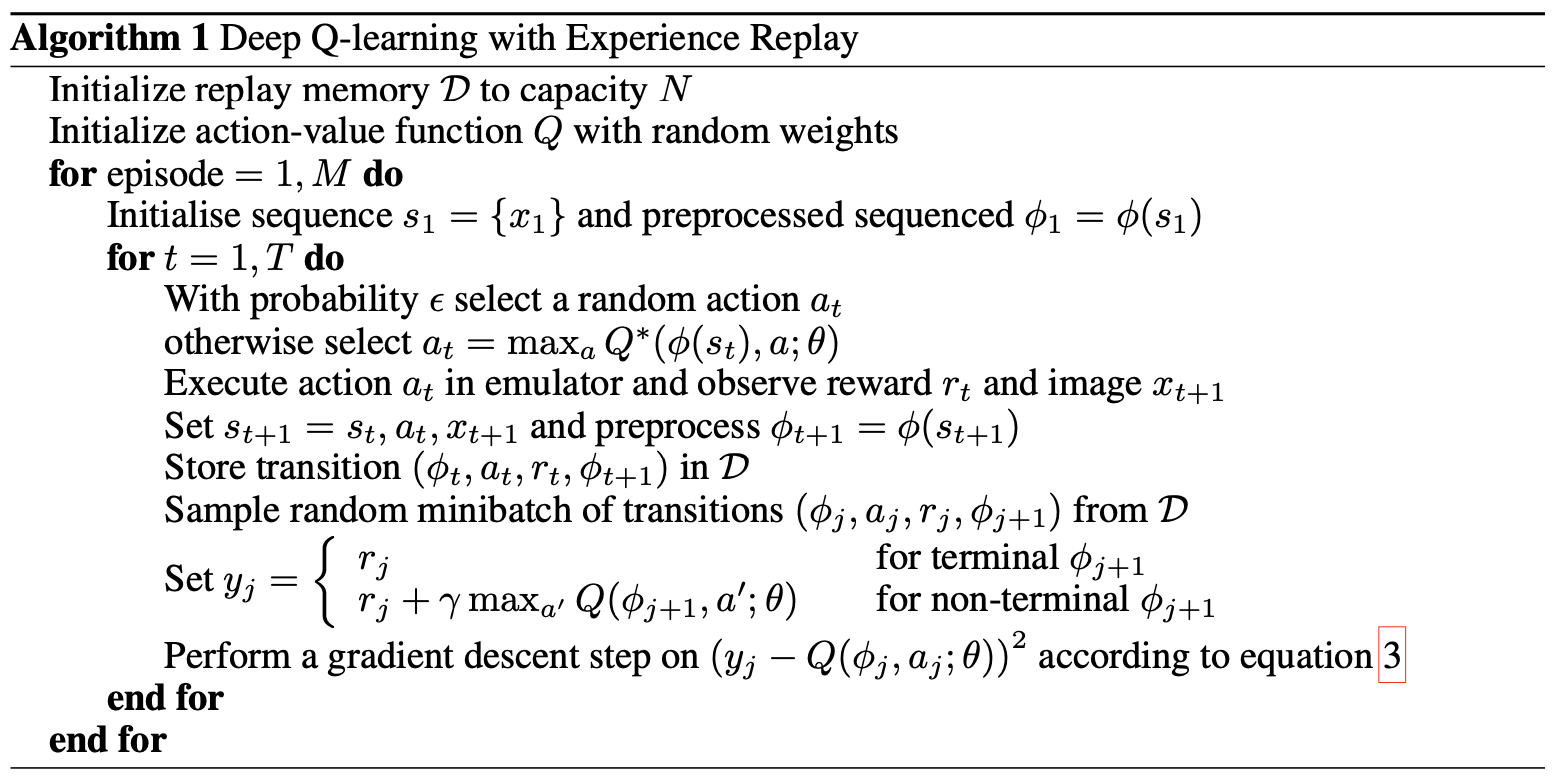
Algorithm 1, reproduced above from Mnih et al. (2013), follows this sequence:
- Initialize replay memory with a fixed capacity.
- Initialize the Q-network with random weights.
- Start an episode and construct the initial preprocessed observation history.
- Choose an action using -greedy exploration.
- Execute the action in the emulator and observe its reward and the next image.
- Extend the history, preprocess it, and store the transition in replay memory.
- Sample a random minibatch of stored transitions.
- For a terminal transition, use the observed reward as the target. Otherwise, add the discounted maximum predicted Q-value at the next state.
- Take a gradient step to reduce .
- Repeat through the episode and subsequent episodes.
Written explicitly, the sampled target is
The source algorithm image writes a maximum where an action is selected. In the explanation, I use for the action itself: gives the value, whereas identifies an action attaining it.
Here, is the preprocessing function that turns a history into a fixed-size representation. Histories keep growing, but the neural network requires a fixed input shape. In these experiments, preprocesses and stacks the most recent four frames.
Preprocessing and the DQN architecture
A raw Atari screen is a RGB image. Processing that directly is relatively expensive, so the paper uses a simple preprocessing sequence:
- Convert RGB to grayscale.
- Downsample to .
- Crop an region covering the playing area.
- Stack the four most recent processed frames to obtain an input.
The network is compact:
| Layer | Configuration |
|---|---|
| Input | |
| First convolution | 16 filters, , stride 4, followed by ReLU |
| Second convolution | 32 filters, , stride 2, followed by ReLU |
| Fully connected hidden layer | 256 ReLU units |
| Output | One linear Q-value output per valid action |
There is an important choice hidden in the output structure. A network could receive both a state and an action and return a single scalar Q-value. To compare all possible actions, we would then need a separate forward pass for each action.
DQN instead receives just the state representation and outputs all action-values at once. A single forward pass supplies everything needed to select the largest one.
A small grid example makes the distinction concrete. Suppose an agent at position has five actions: stay, up, down, left, and right. A scalar-output state-action network would be evaluated five times with five different actions. A state-input network with five outputs produces those five values together.
We still call each component ; the underlying action-value function has not changed. What changes is how efficiently the network evaluates all its actions.
Practical choices in the experiments
The paper evaluates seven Atari games with the same network architecture, the same learning algorithm, and nearly identical hyperparameters. It does not design a new feature extractor or architecture for each game.
I read this as an effort to show that the approach is general across games. It does not mean one jointly trained network plays all seven: the same architecture and training procedure are used to train agents for the individual games.
Since “hyperparameter” has come up, it is useful to distinguish it from a learned parameter. The weights are parameters adjusted by training. Settings such as the learning rate are hyperparameters chosen outside the weight-learning process.
Reward clipping
During training, the method replaces every positive reward with , every negative reward with , and leaves zero unchanged.
Atari games have very different score scales. Clipping limits that variation and makes it easier to reuse the same learning rate across games. The cost is that the agent can no longer distinguish between different magnitudes of positive reward, or between different magnitudes of negative reward. Evaluation uses the original game scores.
Frame skipping
The agent selects an action once every frames and repeats its last action on the intervening frames. This reduces decision-making computation and allows more game progress for similar runtime.
Most games use . Space Invaders uses , because selecting every fourth frame interacts with the lasers' blinking period and can make them invisible to the agent. That is a particularly memorable implementation detail.
How should we judge training progress?
In supervised learning, training loss and validation accuracy give fairly direct ways to monitor progress. In reinforcement learning, the connection is less straightforward.
Episode reward can be very noisy: a small change in the policy may cause a large change in the states it visits. In Figure 2 of the paper, the average reward curves for Breakout and Seaquest fluctuate considerably.
The paper also tracks predicted values on a fixed, held-out set of states collected with a random policy before training. It averages the maximum predicted Q-value across those states. These curves increase much more smoothly than episode reward.
I found this striking. Looking only at rewards can make learning seem erratic, while looking at the learned value estimates reveals a smoother trend. A smoothly increasing prediction is not by itself proof that the prediction is accurate, but it provides a different view of training.
The authors report no divergence in their experiments. They do not establish a general theoretical convergence guarantee. What they show is that, in these experiments, large neural networks could be trained with reinforcement-learning signals and stochastic gradient updates in a stable way.
See Figure 2 and Section 5.1 of the paper for the reward and predicted-value curves discussed here.
Results and significance
The paper reports better performance than the previous approaches it compares against on six of the seven Atari games, and better performance than its human expert on Breakout, Enduro, and Pong.
It does not beat a human on every game. My original notes call out Q*bert, Seaquest, and Space Invaders as examples where longer-term strategy remains difficult. The evaluation also places DQN below the human score on Beam Rider. The six-of-seven claim concerns the overall prior comparison; Table 1 distinguishes several learned baselines and evolutionary-method results.
The achievement is substantial even with those limits. The agents learn from screens, without game-specific hand-designed visual features, using the same architecture and almost the same training settings.
More fundamentally, the paper shows that a deep neural network and Q-learning can work together in practice, with experience replay playing a central role in making that training manageable.
What stood out when I revisited my notes
Looking back through my old Notion notes, three points are what I most want to carry forward.
The first is end-to-end learning: the model learns from pixels to action-values without a person designing an intermediate feature representation for each game.
The second is designing around instability. RL experience is correlated, and its distribution changes as the policy changes. Replay does not eliminate every difficulty, but it substantially changes the conditions under which the network learns.
The third is the Q-network's output structure. Feeding in a state and obtaining values for all actions in one pass looks like a small choice, yet it makes action selection much more efficient. Revisiting the paper helped me notice this detail of the Q architecture more clearly.
I therefore read DQN as a paper in which practical choices fit together to connect deep learning and reinforcement learning. The significance lies in both the CNN's ability to process a game screen and the training structure that makes learning from RL signals work.
Wrapping up
DQN is a CNN-based Q-network that receives processed pixel observations and returns a Q-value for every available action. It combines Q-learning, stochastic gradient updates, -greedy exploration, and experience replay to learn Atari games end to end.
Replay lets experiences be reused, reduces temporal correlation in updates, and softens changes in the training distribution as the policy evolves. These are central to understanding why this combination worked.
More than the statement “deep learning was used for reinforcement learning,” I want to remember why that was difficult and which mechanisms made it practical.
I also hope this reading makes equations feel easier to approach. For this paper, the reading path I would recommend is:
- Identify the central contribution: learning action-values from pixels with a neural network.
- Ask what supports that contribution: replaying past experience reduces the correlation of training samples.
- Follow the experimental implementation: how Atari observations are processed, how the network is organized, and how learning is evaluated.
My original Notion reading notes and lab-meeting material are still linked here, as in the Korean article.
Keep going, and happy studying!