VAEs and the ELBO: learning a distribution instead of a point

This post covers the variational autoencoder (VAE) and the ELBO.

In the last post, we saw what it means for an autoencoder to compress its input and reconstruct it. But spend some time with autoencoders, and a question comes up naturally: reconstruction works, but can we sample from the latent space as easily?

That's exactly where I started to see why the VAE was needed. An autoencoder is strong at compressing to a latent vector and reconstructing, but nothing guarantees the latent space ends up in a shape that's good for sampling. It can reconstruct well and still leave "can it generate new data well?" unanswered. The VAE was built to solve that, and the key to it is the ELBO, the evidence lower bound. Understand the ELBO, and it becomes clear why a VAE isn't just an autoencoder with a few extra equations, but a real step forward as a generative model.

So this post covers what a VAE is, why we need the ELBO, and what each of its terms actually does.

Why an autoencoder isn't enough

An autoencoder maps an input to a latent vector $z$ and back to a reconstruction $\hat{x}$:

That lets it learn a representation for compression and reconstruction. But a plain autoencoder's encoder outputs one fixed latent vector $z$ for each input $x$: every input maps to a single point. Nothing guarantees those points are neatly arranged.

Suppose the training data lands in scattered clumps. The decoder can turn points near training data into plausible outputs, but a randomly chosen $z$ may land in an empty region with no training data nearby, and the decoder may produce something strange. (Think back to the pixel-averaged cat in part 2.) The autoencoder reconstructs well, but doesn't guarantee a latent space that's good for generation.

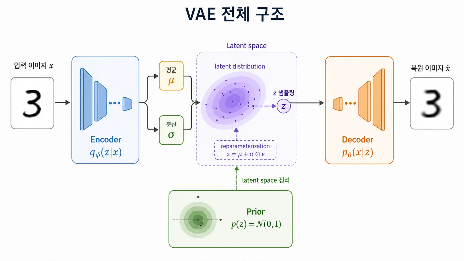
The VAE's key idea is this: train the latent space to fit a distribution we know. That sounds abstract at first, but it turns out to be quite natural. Here's the whole architecture before we dig in:

What's different about a VAE

The basic structure matches an autoencoder:

• Encoder: looks at $x$ and estimates a distribution over the latent variable.
• Decoder: looks at a latent $z$ and generates or reconstructs the data.

The crucial difference is what the encoder outputs. An autoencoder's encoder outputs one fixed vector per input. A VAE's encoder outputs a distribution, usually by predicting a mean and a variance:

So each input maps not to a point in latent space but to a region, a distribution. We then sample $z$ from it and pass it through the decoder:

The encoder no longer produces a single "compressed vector." It learns the latent distribution that can explain the input. For me, that's the first thing to grasp about VAEs: an autoencoder learns a point that represents the input; a VAE learns a distribution that explains it. (Hwalseok Lee's lecture also shows that an autoencoder's latent space can end up arranged differently even for the same training setup.)

A VAE through the generative lens

We can think of real data $x$ as generated from a hidden cause $z$; the latent variable acts like a control knob for producing the data. For MNIST, $z$ might hold slant, stroke thickness, and handwriting style. For cat images, fur pattern, face direction, lighting, and pose. What we ultimately want is to make

large: the probability that our model produces each training example. The trouble is that $p(x)$ is hard to compute. Any $z$ could have produced $x$, so we'd have to account for all of them:

For every possible $z$, add up "how likely this $z$ is" times "how likely it is to produce $x$." Simple to say, very hard in practice, especially for high-dimensional data with a complex latent space. The posterior $p(z \mid x)$ we really want is just as hard. So a VAE uses an approximation $q_\phi(z \mid x)$ in its place. That's the core of variational inference: approximate the intractable posterior $p(z \mid x)$ with a tractable $q_\phi(z \mid x)$. And the objective that trains this approximation well is the ELBO.

Why we need the ELBO

ELBO stands for evidence lower bound. The evidence is $p(x)$. We really want to maximize $\log p(x)$, but can't compute it directly, so we maximize a lower bound we can compute:

The right-hand side is the ELBO. On its own it looks terrifying; it did to me. But there's a clear intuition behind it. We can't get at $\log p(x)$ directly, so we use the encoder's approximation $q_\phi(z \mid x)$ to build a bound that says "it's at least this much," a sort of minimum quality guarantee, and push that bound up. We never touch $\log p(x)$ itself, but we can still train the model in its direction.

Rearranged, the ELBO reveals an even more important relationship:

For me, this is the equation that best shows what the ELBO means. KL divergence is never negative, so the ELBO can never exceed $\log p(x)$. It really is a lower bound. And the smaller the KL term, the closer the ELBO gets to the true evidence.

So the ELBO isn't a makeshift workaround. It's the objective that makes the variational posterior learn well.

The two terms of the ELBO

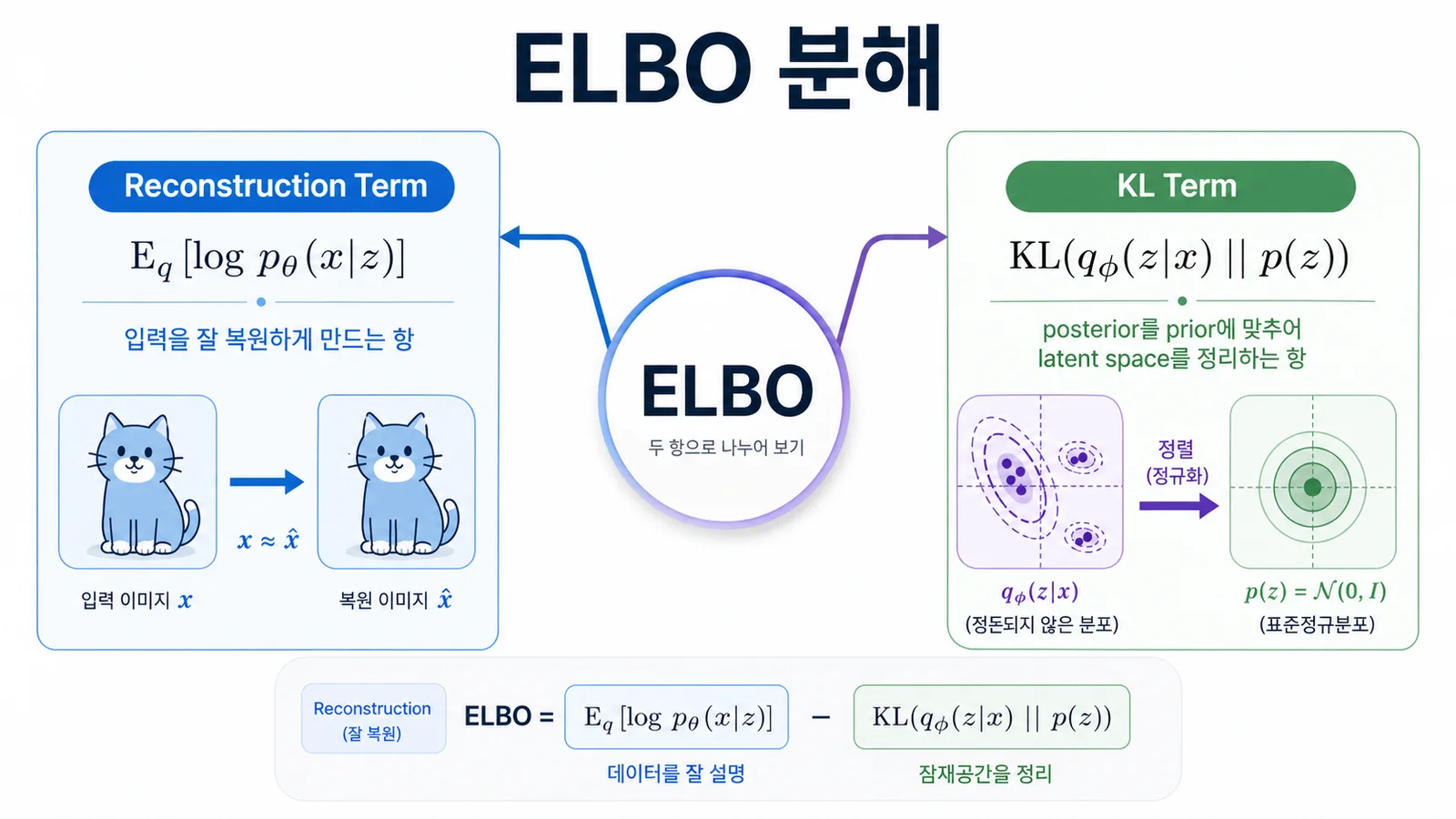
In practice, the ELBO is usually written like this:

This form matters most, because splitting the ELBO into these two terms is the most intuitive way to understand a VAE.

1. The reconstruction term

Sample $z$ from the encoder's latent distribution, and ask the decoder to rebuild the original $x$. This plays almost the same role as an autoencoder's reconstruction loss, except that $z$ is sampled from the distribution $q_\phi(z \mid x)$ rather than being a fixed point. A large value means the decoder explains the data well from the latent variable. In code it can look like MSE under a Gaussian assumption or like BCE under a Bernoulli one. In short, the reconstruction term asks: how well can we regenerate the original $x$ from $z$?

2. The prior matching term

This measures how far the encoder's latent distribution $q_\phi(z \mid x)$ is from the prior $p(z)$ we fixed in advance, usually the standard normal:

The KL term keeps the latent space from scattering wherever it likes. With only a reconstruction term, the encoder could place each input far from the others in latent space: reconstruction would be fine, but sampling would still be hard. As the KL term shrinks, the encoder's latent distributions settle neatly around the standard normal, and after training we can sample straight from the prior and get reasonably plausible outputs. In short:

Put the two together and it's clear what a VAE wants: reconstruct the input well, and keep the latent space organized according to the prior. It's built to get reconstruction and generation at the same time.

The reparameterization trick

Implementation raises one problem. If the encoder outputs a distribution and we sample $z$ from it, the sampling step gets in the way of computing gradients. Backpropagation doesn't flow through it cleanly. So VAEs use the reparameterization trick:

The sampling is moved out of the network into a separate noise variable $\epsilon$. The encoder predicts the mean $\mu$ and standard deviation $\sigma$; the randomness comes from $\epsilon$, drawn from a standard normal. Now $z$ is a differentiable function of $\mu$ and $\sigma$, so gradients can flow back into the encoder.

It feels like a trick at first, but it's essential to making VAEs trainable at all. A VAE doesn't just "use a distribution"; it comes with the machinery to actually learn that distribution.

Generating after training

Generation is surprisingly simple. After training we know the prior, usually a standard normal, so we sample a latent

and decode it:

The encoder isn't needed. Sample from the prior and run the decoder, and that's it. This is the difference from an autoencoder: an autoencoder usually needs an input to produce a latent vector, while a VAE can sample latents without any input because its prior is organized. That's what makes it a better fit as a generative model.

Strengths and limits

Because a VAE's latent space is relatively well organized, interpolation and sampling often behave naturally: nudge the latent vector a little, and the output changes smoothly. We can hope for a semantically meaningful latent space, which is a big plus for a generative model. It also handles distributions explicitly, so it has a probabilistic interpretation, and the ELBO gives a fairly clean reading of the training objective.

It has limits too. The best known is that its outputs can come out blurry. Its expressiveness can also be limited by the latent dimension, the prior, and how the posterior is approximated; if the posterior is restricted to a simple Gaussian family, it may not approximate the true posterior well. The VAE is an important generative model, but not one that solves everything.

Summary

• A VAE compresses and reconstructs like an autoencoder, but the key difference is that it learns a latent distribution, not a single latent point.
• The objective that organizes this distribution around the prior while keeping reconstruction good is the ELBO.
• The ELBO splits into a reconstruction term and a prior matching term; together they aim for reconstruction and samplability at once.
• The reparameterization trick is what lets this probabilistic structure actually be trained.

To me, the VAE is one of the clearest illustrations of how a generative model handles probability distributions before we get to diffusion. With this, the background part of the series is essentially done. Next, we move to paper reading and look at diffusion from a unified perspective.