Today, let's read World Models (Ha & Schmidhuber, 2018).
Paper: World Models. The authors also provide an interactive article and demonstrations.
Figure credit: the paper figures reproduced below are unaltered excerpts from Ha and Schmidhuber (2018), reproduced for commentary. Copyright remains with the respective rights holders. Paper Figure 1 reproduces artwork from Scott McCloud's Understanding Comics (1993), as credited in the paper; the artwork is © Scott McCloud.
World models, sometimes discussed under the broader label of world foundation models, have been drawing a lot of attention. Researchers such as Yann LeCun and Fei-Fei Li, as well as NVIDIA, have pointed to them as a promising direction. I also have a personal reason for being interested: the first paper I wrote borrowed the world-model concept.
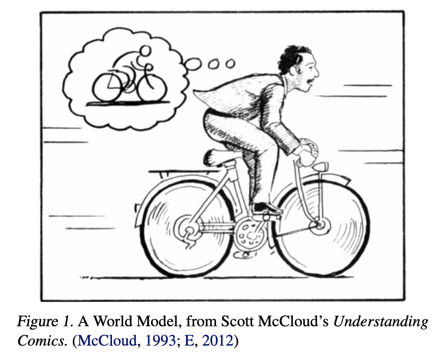
The idea in one sentence is to learn the environment itself as a generative model, then train an agent inside it. Instead of running the actual game, the agent learns inside a dream generated by the model, and we bring that policy back into the real environment.
The VAE from the foundations posts appears as a component. The policy and reward ideas from the reinforcement-learning series return, too. And there is an interesting contrast with Diffusion Policy, which I read just before this.
There are very few equations in this paper. Let's focus on the ideas as we go.
1. We do not remember the whole world
The introduction begins with human mental models. The world in our heads is not the real world itself: it is a model made from selected concepts and the relationships between them.
The authors add another point, citing research suggesting that even what we perceive right now is strongly influenced by the future our internal model predicts.
Their example is baseball. A batter facing a roughly 160 km/h fastball has less time to react than visual information takes to reach the brain. The paper attributes our ability to hit it to an instinctive prediction of when and where the ball will arrive.
Here is how I understood that, with a little interpretation of my own. Diffusion Policy and many other policies calculate actions from observations. In that sense, the immediate input is what was just observed. The baseball example makes me think about the limit of relying on that input alone: a human swings toward a predicted position, even though the ball has not yet been observed there, using trained intuition and technique. This is an intuition for the paper's motivation, rather than a claim that observation-conditioned policies can never learn anticipatory behavior.
I think that sentence captures the design philosophy of the whole paper. The CarRacing experiment later puts numbers behind it.
2. Why separate the world model and controller?
Large RNNs can learn rich representations of space and time. Yet much model-free reinforcement-learning research uses small networks with relatively few parameters.
The authors point to the credit assignment problem. In reinforcement learning, it is difficult to work out how much a particular action contributed to a reward received later. Learning millions of weights from that signal alone is hard, so smaller networks that let researchers iterate quickly are often the practical choice.
What can we do instead? The paper splits the agent into two parts:
- A large world model learns the environment through unsupervised learning. A differentiable loss lets us train it efficiently with backpropagation. The full world model consists of the VAE and MDN-RNN.
- A small controller chooses actions using the representations the world model provides. Its small parameter count keeps credit assignment within a small search space.
Here are the parameter counts for CarRacing:
| Component | Parameters |
|---|---|
| VAE | 4,348,547 |
| MDN-RNN | 422,368 |
| Controller | 867 |
The controller accounts for less than 0.02% of the total. Almost all the agent's representational capacity sits in the world model, while the part that actually chooses an action is a single linear layer. That is deliberate.
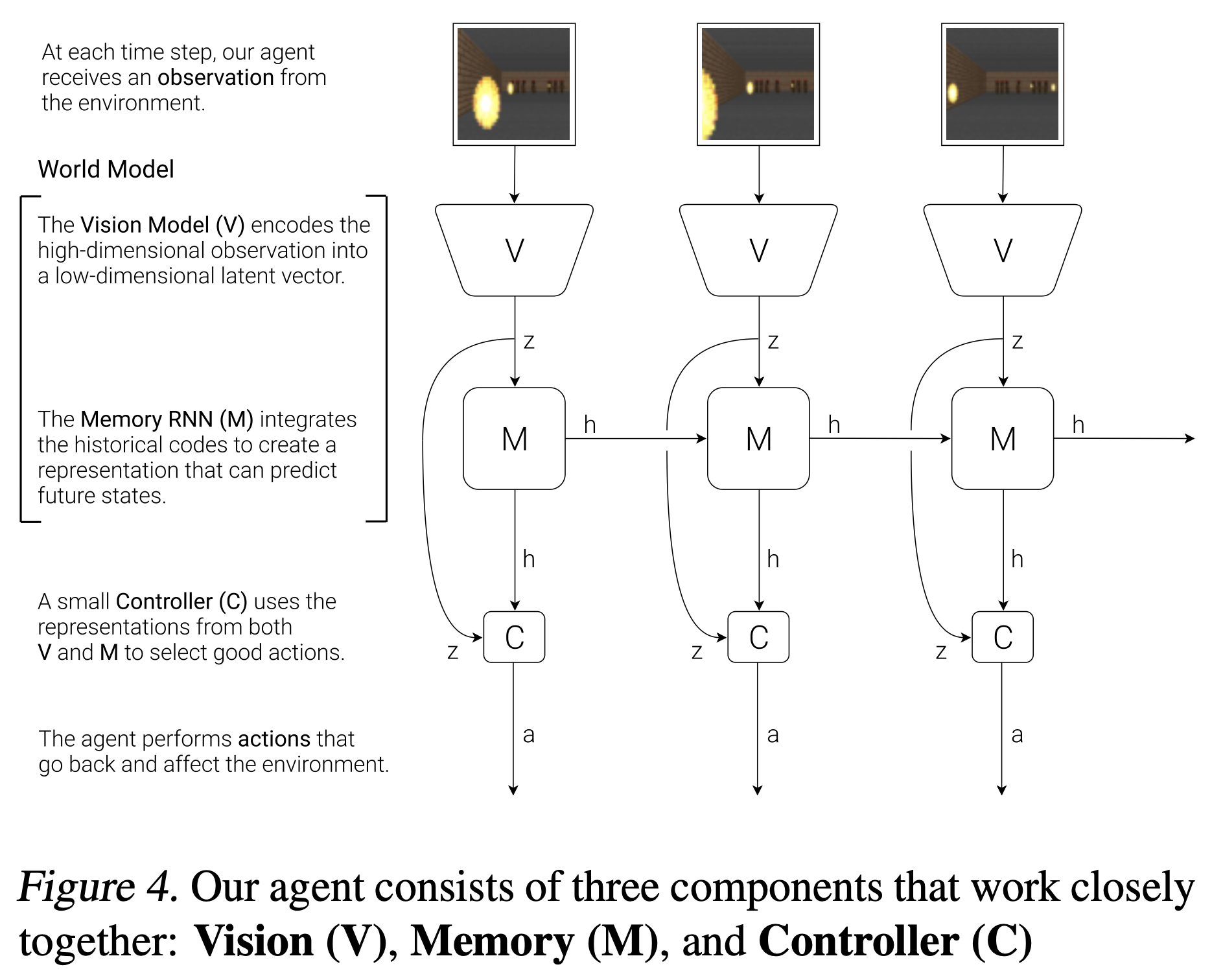
2.1. V (Vision): compressing space
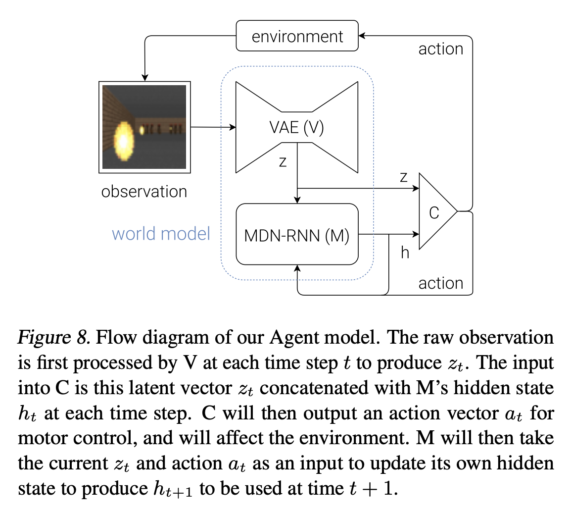
The three components are Vision (V), Memory (M), and Controller (C).
V compresses the observation image at each time step into a small latent vector. This is where the VAE comes in.
It is the same structure we saw in the foundations posts: four convolutional layers encode a image into and , a latent is sampled, and four transposed-convolutional layers reconstruct the image. The latent dimension is 32 for CarRacing and 64 for Doom.
The appendix explains why they chose a VAE instead of an ordinary autoencoder. Enforcing a Gaussian prior limits how much information each frame can carry. At the same time, that prior makes the model more robust to unrealistic vectors produced by M.
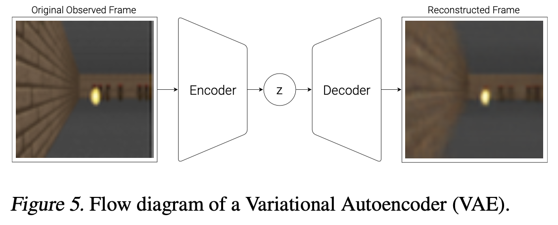
In the autoencoder post, we saw that the prior helps organize the latent space, which is useful when generating samples. That matters here because, when we visualize a dream, we feed the produced by M into the decoder. If the latent space is poorly organized, even a small move away from the encoded training samples can produce a broken reconstruction.
An ordinary autoencoder does not enforce that same latent distribution; its arrangement can differ between training runs. As I mentioned in the earlier post, Hwal-seok Lee's lecture Everything about Autoencoders illustrates this well. If that point still feels abstract, watch the lecture from about 43 minutes; seeing it makes it much easier to understand.
This is the prior-matching term from the VAE and ELBO post earning its keep.
2.2. M (Memory): compressing time
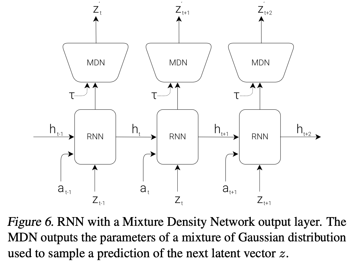
V compresses a moment. M compresses what happens over time. Its job is to predict the next latent:
Here, is the action at time , and is the RNN's hidden state.
There is an important distinction: M predicts the next frame's latent vector, rather than the next frame's pixels. This is what makes learning inside a dream practical. We can simulate entirely in latent space without rendering images.
There is another important detail. M outputs a probability distribution, rather than one deterministic value of .
The architecture is an MDN-RNN: an LSTM with a Mixture Density Network output layer. It represents the next latent distribution using a mixture of Gaussians. The experiments use five mixture components and a diagonal form that does not model correlations between latent dimensions.
I had a question here: if the VAE already encodes a frame with a single diagonal Gaussian, why do we need a mixture?
The paper raises and answers the same question. Discrete modes are useful because the environment contains discrete random events. A monster either shoots a fireball at this moment or stays put; those are distinct events, rather than a continuous blend of the two.
A single Gaussian may be enough to encode an individual frame, while a mixture helps model the logic that connects frames.
The latent-space picture from the autoencoder lecture also gives a useful visual intuition for several Gaussian-shaped clusters. That visual resemblance is helpful, though an ordinary autoencoder's latent distribution is not automatically an MDN.
Finally, a sampling temperature controls model uncertainty. This parameter ends up playing a surprisingly large role.
2.3. C (Controller): a single linear layer
Now for the controller. This is where the paper's only numbered equation appears:
This is Equation (1) in the paper. Concatenate the compressed current observation with the RNN hidden state , multiply by a matrix, add a bias, and you have the action.
There is no hidden layer in C. The equation is a linear map; the implementation then applies the environment's action-output mappings.
The authors explicitly say they made C this small so that most of the agent's complexity would reside in the world model. They want dynamics and the relationships needed to represent the environment to be learned there.
There is a practical benefit, too. With so few controller parameters, we can use an optimizer that does not require a differentiable loss. The paper uses CMA-ES, an evolution strategy, to find and .
CMA-ES works well for search spaces containing up to a few thousand parameters, so an 867-parameter controller fits comfortably. The appendix uses a population of 64. Each candidate performs 16 rollouts with different random initial seeds, and its average cumulative reward becomes its fitness. For CarRacing, training ran for 1,800 generations.
2.4. Putting the three together
In words, Figure 8 and the rollout pseudocode describe this loop:
- Receive observation from the environment and encode it with V to get .
- Concatenate and M's current hidden state , pass them to C, and obtain action .
- Apply to the environment, receiving a reward and the next observation.
- Feed and into M to update its hidden state to .
An interesting detail is that, in the CarRacing experiment, the world model knows nothing about the reward. V and M only compress and predict observation sequences. Only C has access to reward information.
Learning how the world behaves and learning how to achieve a goal are separate jobs.
3. CarRacing: does the controller get h_t?
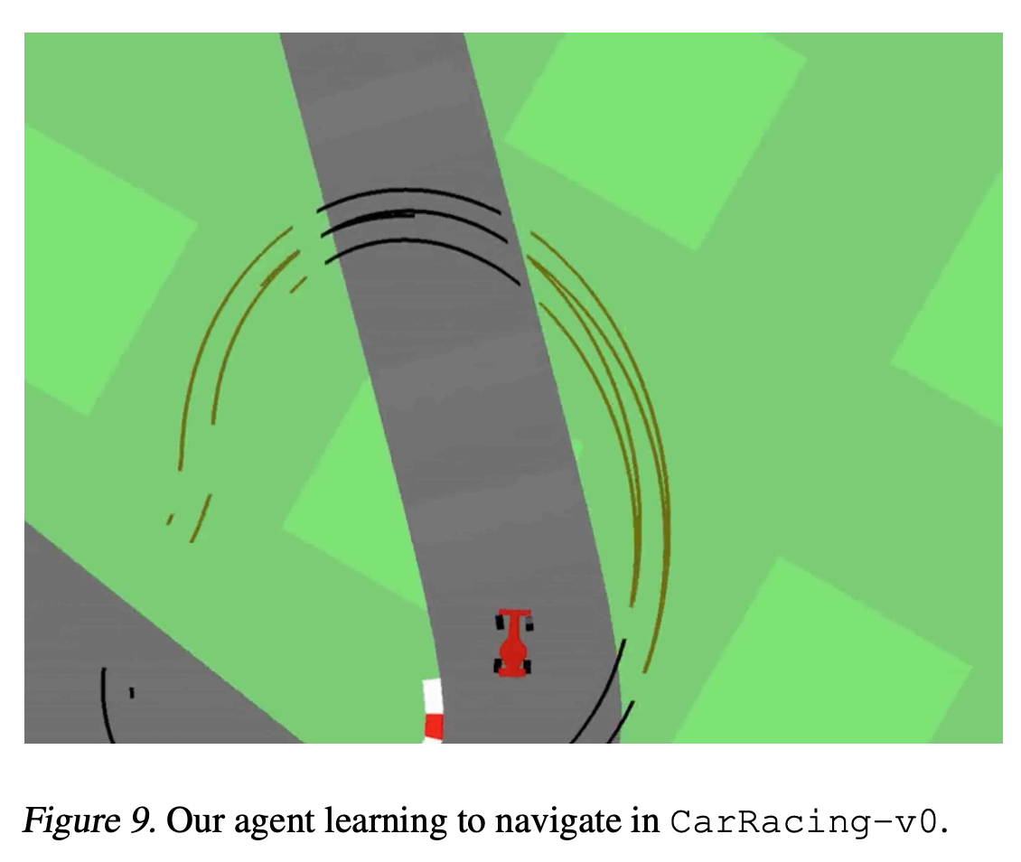
The first experiment uses CarRacing-v0. A new track is generated randomly for each trial, and visiting more track tiles in less time earns reward.
The procedure is:
- Collect 10,000 rollouts using a random policy.
- Train the VAE on those frames to obtain .
- Train the MDN-RNN using the encoded latents and recorded actions.
- Define the controller and use CMA-ES to maximize cumulative reward.
The key comparison is whether the controller receives .
With only , it sees a compressed version of the current frame. It does not get M's learned temporal representation. With , it also gets the state M maintains to predict , which contains information useful for anticipating what comes next.
The paper's Table 1 reports:
| Controller inputs and architecture | Score, mean ± standard deviation |
|---|---|
| V only | 632 ± 251 |
| V only, with an added hidden layer | 788 ± 141 |
| V and M | 906 ± 21 |
The environment counts as solved when the mean score exceeds 900 over 100 consecutive trials. The authors describe theirs as the first solution known to them. The A3C variants in the comparison scored roughly 591–652; the previous leaderboard best was 838 ± 11.
What struck me more than the mean was the standard deviation. Adding M reduces it from 251 to 21. That agrees with the paper's description: the agent using only wobbles and loses the track at sharp bends.
The authors return to the baseball analogy here. Because contains the information used to construct a distribution over possible futures, the agent can use that representation directly without explicitly rolling those futures forward. C receives , rather than a sampled future latent.
A model trained to predict the future makes driving steadier, even without explicit planning.
4. VizDoom: learning inside a dream
This is where the paper's central claim really comes into focus.
In CarRacing, a policy trained in the real environment also works to some extent inside a dream. Can we reverse that: learn inside the dream and transfer the policy into reality?
The task is VizDoom's Take Cover. Monsters on the opposite side fire projectiles, and the agent must dodge them for as long as possible.
There is no explicit reward signal, so the authors define cumulative reward as the number of time steps survived. A mean above 750 steps over 100 consecutive rollouts counts as solving the task.
There is one decisive difference from CarRacing. M now predicts not only the next latent but also whether the agent dies at the next frame:
That small addition changes a lot. If M can produce the next observation representation and determine termination, it can supply the transitions and episode endings needed for this survival task. Reward follows from the number of steps survived.
The authors wrap M in a Gym environment interface and train the agent in this generated environment instead of the real game.
V is unnecessary during dream training: there is no reason to create pixels, so the whole process stays in latent space. V is used again to encode real observations when the policy is transferred back.
The results are roughly:
- Inside the virtual environment: 900 steps.
- After transfer to the actual environment: 1,100 steps.
Both comfortably exceed 750. More surprisingly, the agent does better in reality than inside the dream.
The paper's explanation is that the virtual environment was deliberately made noisier and more uncertain than the real one. An agent that survives that harsher nightmare fares well in the cleaner actual environment.
The authors also spell out what M has learned. From raw images of random episodes, it learns to approximate game logic, enemy behavior, physics, and even the rendered appearance of a 3D environment. A left action moves the agent left, walls block movement, multiple monsters' fireballs continue on their own trajectories, and the model judges whether one hits the agent.
4.5. Then the agent started cheating in its dream
Personally, this was the most entertaining part of the paper.
In early experiments, the authors noticed something strange. If the agent moved in a particular way, monsters in the generated environment would never fire a single projectile during some rollouts. Even when a fireball seemed about to appear, the agent could move and extinguish it, almost like a superpower.
Why? The authors give two explanations.
First, the world model is only an approximate probabilistic model. It can generate trajectories that violate the real environment's rules. I liked their analogy: a child can learn that things fall downward and still imagine a superhero who flies.
Second, using M as the environment gives the controller access to M's entire hidden state. It is rather like handing a player the internal state and memory of the game engine, beyond the screen a player normally sees.
The agent can then find actions that exploit those internal dynamics to maximize reward. It does not directly write to memory; its actions influence a model whose internal state it can observe.
This is a fundamental weakness of learning a policy inside learned dynamics: an adversarial policy may exploit the model's mistakes. It looks excellent inside the model and fails in reality, often because it visits states far from the training distribution, where the model is inaccurate.
The authors suggest this may help explain why earlier approaches generally did not replace the real environment completely with a learned dynamics model.
Making the dream deliberately harder
The solution is interesting. An MDN-RNN models a distribution of possible outcomes, rather than a single deterministic future. That is the first line of defense. Even a deterministic actual environment can be approximated as a stochastic one.
Temperature adds another control. Raising it makes the dream more uncertain: fireballs travel less predictably, and the agent may sometimes die for no clear reason. Temperature becomes a knob controlling the trade-off between realism and exploitability.
Table 2 makes the effect concrete:
| Temperature | Virtual score | Actual score |
|---|---|---|
| 0.10 | 2086 ± 140 | 193 ± 58 |
| 0.50 | 2060 ± 277 | 196 ± 50 |
| 1.00 | 1145 ± 690 | 868 ± 511 |
| 1.15 | 918 ± 546 | 1092 ± 556 |
| 1.30 | 732 ± 269 | 753 ± 139 |
| Random policy | N/A | 210 ± 108 |
| Gym leaderboard best | N/A | 820 ± 58 |
Data: Ha and Schmidhuber (2018), Table 2. Scores are survival time steps, reported as mean ± standard deviation.
The first row says it all. At , the agent gets a near-perfect 2086 in its dream, then performs worse than a random policy in the real environment.
The paper explains this as mode collapse. With temperature too low, M behaves almost like a deterministic LSTM and fails to transition into the mixture mode that generates fireballs. The monsters in that dream do not shoot, whatever the agent does. A policy learned in that world has little chance in the real one.
Raise temperature too far, though, and the dream becomes so difficult that the agent cannot learn anything. It is a hyperparameter that needs tuning.
Temperature also changes the kind of strategy the agent learns. The highest actual mean occurs at . Increasing it to 1.30 reduces the mean but also substantially reduces the variance, producing a less risky strategy.
5. Harder environments: iterative training
The authors acknowledge that their tasks are relatively simple. A random policy collected enough data to learn a useful world model.
In harder environments, some parts of the world only become accessible after the agent has already learned to act competently. Random exploration will not reach them.
They therefore propose an iterative procedure:
- Initialize M and C with random parameters.
- Run rollouts in the actual environment, saving actions and observations.
- Train M on that data, then train C inside M to optimize expected reward.
- Return to step 2 if the task is not yet complete.
The paper's more general version of step 3 models
including the next observation, reward, action, and termination signal. This is the procedure shown in the excerpt in my Korean original; it is a proposal for more complicated tasks, rather than the exact latent-only setup used above.
One additional idea stood out to me. If M predicts the next-frame distribution poorly, the agent may be in an unfamiliar part of the world. We can reuse that prediction failure as a curiosity signal, encouraging the agent to visit places it does not yet understand. The new data can then improve the world model.
The paper describes reversing the model-training objective for exploration. The direction matters: M learns to reduce prediction error, while the exploring controller is encouraged to seek it. A reward based on a positive prediction loss would therefore increase with that loss.
The authors look further ahead, too. As iterations continue, M could absorb motor skills C has already learned, freeing the small controller to focus on higher-level skills. This is a research direction, rather than a result demonstrated by these experiments.
6. Limitations the paper itself identifies
The discussion does not only list advantages.
The first limitation is training V separately. An unsupervised VAE does not know which details matter for the task, so it spends capacity on irrelevant information.
The examples are memorable:
- In Doom, it reconstructs the relatively unimportant brick pattern on the side walls well.
- In CarRacing, it struggles to reconstruct the road tiles that actually matter.
Joint training with an M that predicts reward could help V focus on task-relevant details. The trade-off is that the representation may become harder to reuse for other tasks.
The second limitation is world-model capacity. We can store a great deal of experience externally, but an LSTM cannot necessarily absorb it all into its weights. Catastrophic forgetting is another problem.
The third is the simulation approach itself. It rolls possible futures forward one step at a time. It does not perform human-like hierarchical planning or abstract reasoning that ignores unnecessary details of space and time.
What I took away from reading it
I read this immediately after Diffusion Policy, and I wanted to point out a comparison:
- Diffusion Policy represents the policy as a generative model. Given observations, it generates a distribution of actions.
- World Models represents the environment as a generative model. Given an action and the current representation, it generates a distribution of the next observation's latent representation.
Both use generative models for control. They differ in what they generate.
Both also made me think about what happens away from the learned distribution. Diffusion Policy repeatedly takes in new observations through receding-horizon control. World Models makes the dream deliberately harder by increasing temperature. These are different responses to uncertainty; neither eliminates distribution shift in general.
Wrapping up
Today we read World Models. It separates an agent into a large world model, made from a VAE and MDN-RNN, and a tiny controller: a single linear layer with 867 parameters in CarRacing.
The world model learns to compress space and time through unsupervised learning. The controller learns with CMA-ES using those representations.
I found the architecture particularly impressive: the authors deliberately arrange the components so that the MDN-RNN learns the dynamics. The finding that a more uncertain dream can produce better real-world behavior also stayed with me.
In the next post, I want to follow this thread and look at how world-model approaches developed afterward.
Keep going, and see you next time!